Fully coherent search using MCMC

In this example, we will show the basics of setting up and running a fully-coherent MCMC search. This is based on the example fully_coherent_search_using_MCMC.py. We will run the search on the basic data generated in the make_fake_data example.

First, we need to import the search tool, in this example we will use the MCMCSearch, but one could equally use MCMCGlitchSearch with nglitch=0. To import this,

from pyfstat import MCMCSearch

Next, we define some variables defining the exact parameters of the signal in the data, and the start and end times:

F0 = 30.0
F1 = -1e-10
F2 = 0
Alpha = np.radians(83.6292)
Delta = np.radians(22.0144)
tref = 362750407.0

tstart = 1000000000
duration = 100*86400
tend = tstart = duration

Now, we need to specify our prior. This is a dictionary containing keys for each variable (in the MCMCSearch these are F0, F1, F2, Alpha, and Delta). In this example, we choose a uniform box in F0 and F1:

theta_prior = {'F0': {'type': 'unif', 'lower': F0*(1-1e-6), 'upper': F0*(1+1e-6)},
               'F1': {'type': 'unif', 'lower': F1*(1+1e-2), 'upper': F1*(1-1e-2)},
               'F2': F2,
               'Alpha': Alpha,
               'Delta': Delta
               }

Each key and value of the theta_prior contains an instruction to the MCMC search. If the value is a scalar, the MCMC search holds these fixed (as is the case for F2, Alpha, and Delta here). If instead the value is a dictionary describing a distribution, this is taken as the prior and the variable is simulated in the MCMC search (as is the case for F0 and F1). Note that for MCMCSearch, theta_prior must contain at least all of the variables given here (even if they are zero), and if binary=True, it must also contain the binary parameters.

Next, we define the parameters of the MCMC search:

ntemps = 4
log10temperature_min = -1
nwalkers = 100
nsteps = [1000, 1000]

These can be considered the tuning parameters of the search. A complete discussion of these can be found here.

Passing all this to the MCMC search, we also need to give it a label, a directory to save the data, and provide sftfilepath, a string matching the data to use in the search

mcmc = MCMCSearch(label='fully_coherent_search_using_MCMC', outdir='data', 
                  sftfilepath='data/*basic*sft', theta_prior=theta_prior,
                  tref=tref, tstart=tstart, tend=tend, nsteps=nsteps,
                  nwalkers=nwalkers, ntemps=ntemps,
                  log10temperature_min=log10temperature_min)

To run the simulation, we call

mcmc.run()

This produces two .png images. The first is the position of the walkers during the simulation: 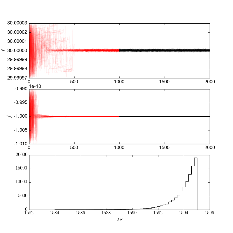This shows (in red) the position of the walkers during the burn-in stage. They are initially defuse (they start from positions randomly picked from the prior), but eventually converge to a single stable solution. The black is the production period from which posterior estimates are made. The bottom panel is a histogram of twoF, split for the production period. Note that, early on there are multiple modes corresponding to other peaks, by using the parallel tempering, we allow the walkers to explore all of these peaks and opt for the strong central candidate.

To get posteriors, we call

mcmc.plot_corner()

which produces a corner plot 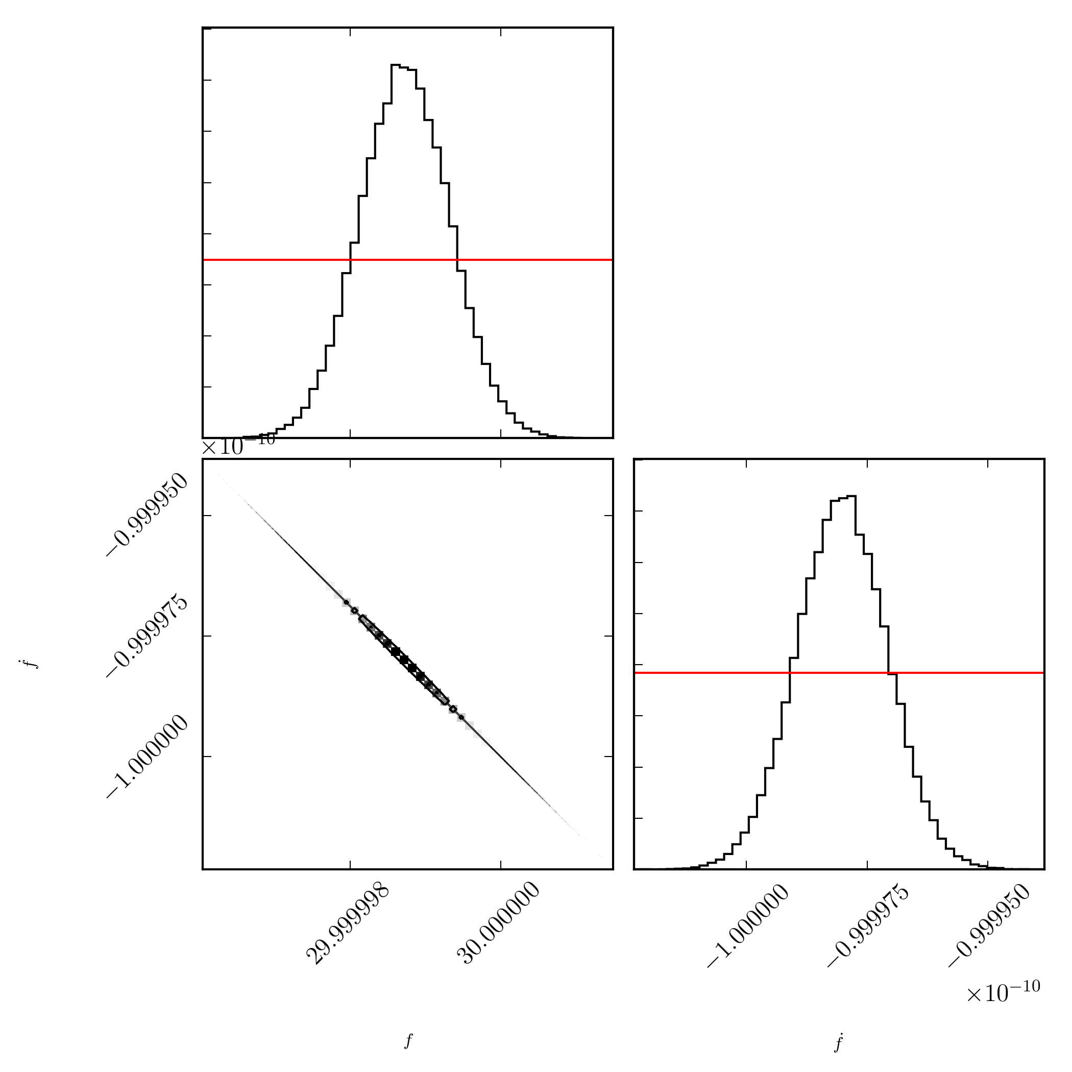illustrating the tightly constrained posteriors on F0 and F1 and their covariance. Furthermore, one may wish to get a summary which can be printed to the terminal via

mcmc.print_summary()

which gives the maximum twoF value, median and standard-deviation, in this case this is

Summary:
theta0 index: 0
Max twoF: 1771.50622559 with parameters:
  F0         = 2.999999874e+01
  F1         = -9.999802960e-11

Median +/- std for production values
  F0         = 2.999999873e+01 +/- 6.004803009e-07
  F1         = -9.999801583e-11 +/- 9.359959909e-16